Neural Networks – algorithms and applications

By Fiona Nielsen 4i

12/12-2001

Supervisor: Geert Rasmussen Niels Brock Business College

Neural Networks is a field of Artificial Intelligence (AI) where we, by inspiration from the human brain, find data structures and algorithms for learning and classification of data.

Many tasks that humans perform naturally fast, such as the recognition of a familiar face, proves to be a very complicated task for a computer when conventional programming methods are used. By applying Neural Network techniques a program can learn by examples, and create an internal structure of rules to classify different inputs, such as recognising images.

This document contains brief descriptions of common Neural Network techniques, problems and applications, with additional explanations, algorithms and literature list placed in the Appendix.

Keywords:

Artificial Intelligence, Machine Learning, Algorithms, Data mining, Data Structures, Neural Computing, Pattern Recognition, Computational Statistics.

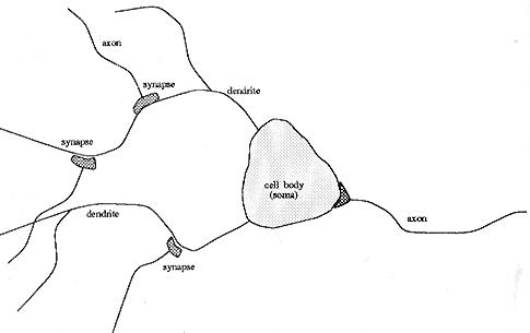
The simple neuron model is made from studies of the human brain neurons. A neuron in the brain receives its chemical input from other neurons through its dendrites. If the input exceeds a certain threshold, the neuron fires its own impulse on to the neurons it is connected to by its axon. Below is a very simplified figure as each of the neurons of the brain is connected to about 10000 other neurons.

Illustration 1 The Neuron

The simple perceptron models this behaviour in the following way. First the perceptron receives several input values (x₀ - x_n). The connection for each of the inputs has a weight (w₀ - w_n) in the range 0-1. The Threshold Unit then sums the inputs, and if the sum exceeds the threshold value, a signal is sent to output. Otherwise no signal is sent.

The perceptron can learn by adjusting the weights to approach the desired output.

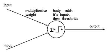
Illustration 2 The Perceptron

With one perceptron, it is only possible to distinguish between two pattern classes, with the visual representation of a straight separation line in pattern space (Illustration 8 Pattern Space).

Algorithm

The perceptron can be trained by adjusting the weights of the inputs with Supervised Learning. In this learning technique, the patterns to be recognised are known in advance, and a training set of input values are already classified with the desired output. Before commencing, the weights are initialised with random values. Each training set is then presented for the perceptron in turn. For every input set the output from the perceptron is compared to the desired output. If the output is correct, no weights are altered. However, if the output is wrong, we have to distinguish which of the patterns we would like the result to be, and adjust the weights on the currently active inputs towards the desired result. (Formula 2 SLP Adapt Weights)

Perceptron Convergence Theorem

The perceptron algorithm finds a linear discriminant function in finite iterations if the training set is linearly separable. [Rosenblatt 1962]

The learning algorithm for the perceptron can be improved in several ways to improve efficiency, but the algorithm lacks usefulness as long as it is only possible to classify linear separable patterns.

Building on the algorithm of the simple Perceptron, the MLP model not only gives a perceptron structure for representing more than two classes, it also defines a learning rule for this kind of network.

The MLP is divided into three layers: the input layer, the hidden layer and the output layer, where each layer in this order gives the input to the next. The extra layers gives the structure needed to recognise non-linearly separable classes.

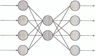
Illustration 3 The Multi Layer Perceptron

Algorithm

The threshold function of the units is modified to be a function that is continuous derivative, the Sigmoid function(Formula 4 The Sigmoid Function). The use of the Sigmoid function gives the extra information necessary for the network to implement the back-propagation training algorithm.

Back-propagation works by finding the squared error (the Error function) of the entire network, and then calculating the error term for each of the output and hidden units by using the output from the previous neuron layer. The weights of the entire network are then adjusted with dependence on the error term and the given learning rate. (Formula 6 MLP Adapt weights)

Training continues on the training set until the error function reaches a certain minimum. If the minimum is set too high, the network might not be able to correctly classify a pattern. But if the minimum is set too low, the network will have difficulties in classifying noisy patterns.

Comparison SLP MLP

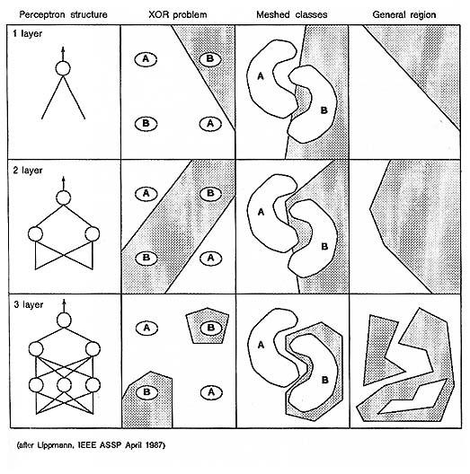
The MLP can be compared to the single layer perceptron by reviewing the XOR classification problem. The SLP can only perform the simple binary operations. When advancing to using several unit layers we can construct the XOR (Illustration 9 Decision regions).

Below is an example of a MLP solution to the XOR problem in 2D space.

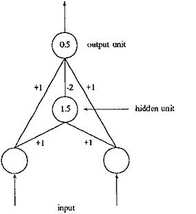
Illustration 4 A MLP Solution to XOR

Even though we here find the MLP a much more convenient classification network, it introduces a new problem: The MLP network is not guaranteed to find convergence!

The MLP risks ending up in a situation where it is impossible to learn to produce the right output. This state of a MLP is called a local minimum (see Problems using Neural Networks).

Many advanced algorithms have been invented since the first simple neural network. Some algorithms are based on the same assumptions or learning techniques as the SLP and the MLP. A very different approach however was taken by Kohonen, in his research in self-organising networks.

The Kohonen self-organising networks have a two-layer topology. The first layer is the input layer, the second layer is itself a network in a plane. Every unit in the input layer is connected to all the nodes in the grid in the second layer. Furthermore the units in the grid function as the output nodes.

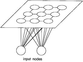
Illustration 5 The Kohonen topology

The nodes in the grid are only sparsely connected. Here each node has four immediate neighbours.

Algorithm

The network (the units in the grid) is initialised with small random values. A neighbourhood radius is set to a large value. The input is presented and the Euclidean distance between the input and each output node is calculated. The node with the minimum distance is selected, and this node, together with its neighbours within the neighbourhood radius, will have their weights modified to increase similarity to the input. The neighbourhood radius decreases over time to let areas of the network be specialised to a pattern. (Formula 10 Kohonen Calculate Distances and Formula 11 Kohonen Update Weights)

The algorithm results in a network where groups of nodes respond to each class thus creating a map of the found classes.

The big difference in the learning algorithm, compared with the MLP, is that the Kohonen self-organising net uses unsupervised learning. But after the learning period when the network has mapped the test patterns, it is the operators responsibility to label the different patterns accordingly.

The Hopfield net is a fully connected, symmetrically weighted network where each node functions both as input and output node. The idea is that, depending on the weights, some states are unstable and the net will iterate a number of times to settle in a stable state.

The net is initialised to have a stable state with some known patterns. Then, the function of the network is to receive a noisy or unclassified pattern as input and produce the known, learnt pattern as output.

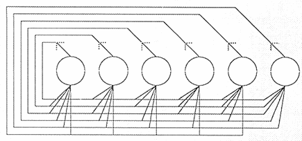
Illustration 6 The Hopfield topology

Algorithm

The energy function for the network is minimised for each of the patterns in the training set, by adjusting the connection weights. An unknown pattern is presented for the network. The network iterates until convergence. (Formula 14 Hopfield Iterate until convergence)

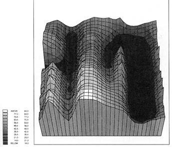
The Hopfield net can be visualised by means of the Energy Landscape (Illustration 10 The Energy Landscape), where the hollows represent the stored patterns. In the iterations of the Hopfield net the energy will be gradually minimised until a steady state in one of the basins is reached.

An even newer algorithm is the Bumptree Network which combines the advantages of a binary tree with an advanced classification method using hyper ellipsoids in the pattern space instead of lines, planes or curves. The arrangement of the nodes in a binary tree greatly improves both learning complexity and retrieval time.

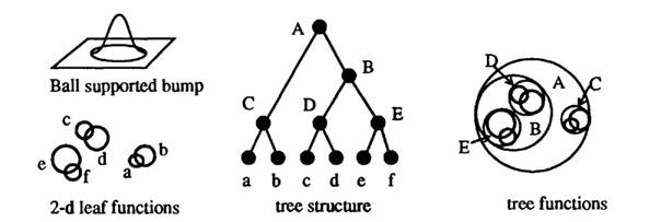
Illustration 7 An example visualisation of a 2d bumptree network

Neural Networks are successfully being used in many areas often in connection with the use of other AI techniques.

A classic application for NN is image recognition. A network that can classify different standard images can be used in several areas:

• Quality assurance, by classifying a metal welding as whether is holds the quality standard.

• Medical diagnostics, by classifying x-ray pictures for tumor diagnosis.

• Detective tools, by classifying fingerprints to a database of suspects.

A well known application using image recognition is the Optical Character Recognition (OCR) tools that we find available with the standard scanning software for the home computer. Scansoft has had great success in combining NN with a rule based system for correctly recognising both characters and words, to get a high level of accuracy¹.

All the network topologies and algorithms have their advantages and disadvantages. When it comes to understanding the spoken language the best found solutions use a combination of NN for phoneme recognition and an Expert system for Natural language processing, where neither AI technique can be adapted to solve the problem in whole. Kohonen himself succeeded in creating a 'phonetic typewriter' by using his self-organising networks for the phoneme recognition and a rule base for applying the correct grammar.

Another popular application for NN is Customer Relationship Management(CRM).

Many companys have at the same rate as electronic data storage has become commonplace built up large customer databases. By using Neural Networks for data mining in these databases, patterns however complex can be identified for the different types of customers, thus giving valuable customer information to the company.

One example is the airline reservation system AMT² which could predict sales of tickets in relation to destination, time of year and ticket price. The NN strategy was well suited for the purpose because the system could be updated continuously with the actual sales.

In relation to the recent trends in Management strategies CRM has reached a high priority, because of the prospects of a successful CRM system adding value to the business in terms of not only better prediction of customer needs but also predicting which customers will be the most valuable for the company.

Some rules of thumb exist for evaluating whether a problem is suitable for a Neural Network implementation:

• There must be a large example dataset of the problem in order to be able to train the network.

• The data relationships in the problem are complex and difficult or impossible to program using conventional techniques.

• The output does not need to be exact or numeric.

• The desired output from the system changes over time, so a high flexibility is needed.

Many commercial NN programs exist both for stand-alone or built-in applications.

All the NN in this paper are described in their basic algorithm. Several suggestions for improvements and modifications have been made. One of the well-known problems in the MLP is the local minimum: The net does not settle in one of the learned minima but instead in a local minimum in the Energy landscape (Illustration 10 The Energy Landscape).

Approaches to avoid local minimum:

• The gain term in the weight adaption function can be lowered progressively as the network iterates. This would at first let the differences in weights and energy be large, and then hopefully when the network is approaching the right solution, the steps would be smaller. The tradeoff is when the gain term has decreased the network will take a longer time to converge to right solution. (Formula 6 MLP Adapt weights)

• A local minimum can be caused by a bad internal representation of the patterns. This can be aided by the adding more internal nodes to the network.

• An extra term can be added to the weight adaption: the Momentum term. The Momentum term should let the weight change be large if the current change in energy is large. (Formula 9 MLP Momentum term)

• The network gradient descent can be disrupted by adding random noise to ensure sure the sytem will take unequal steps toward the solution. This solution has the advantage, that it requires no extra computation time.

A similar problem is known in the Hopfield Net as metastable states. That is when the network settles in a state that is not represented in the stored patterns. One way to minimise this is by adjusting the number of nodes in the network(N) to the number of patterns to store, so that the number of patterns does not exceed 0.15N. Another solution is to add a probabilistic update rule to the Hopfield network. This is known as the Boltzman machine.

There are some practical problems applying Neural networks to applications.

It is not possible to know in advance the ideal network for an application. So every time a NN is to be built in an application, it requires tests and experiments with different network settings or topologies to find a solution that performs well on the given application. This is a problem because most NN requires a long training period – many iterations of the same pattern set. And even after many iterations there is no way other that testing to see whether the network is efficiently mapping the training sets. A solution for this might be to adapt newer NN technologies such as the bumptree which need only one run through the training set to adjust all weights in the network. The most commonly used network still seems to be the MLP and the RBF³ even though alternatives exist that can drastically shorten processing time.

In general most NN include complex computation, which is time consuming. Some of these computations could gain efficiency if they were to be implemented on a parrallel processing system, but the hardware implementation raises new problems of physical limits and the NN need for changeability.

Several attempts have been made to optimise Neural Networks using Genetic Algorithms(GA), but as it shows, not all network topologies are suited for this purpose.

How can GA be used in the field of Neural Networks?

How can the Bumptree Network be efficiently optimised using GA?

APPENDIX

The inputs data for Neural Networks are represented using feature vectors. Each element in the vector corresponds to a feature of the input.

All input patterns have the same number n of features, and thus creating a n-dimensional feature space. Feature space is easiest to visualise in the 2-dimensions, see below.

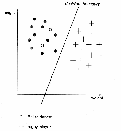
Illustration 8 Pattern Space

The input patterns can be drawn on the graph as (x,y) sets. The values of the axis can be discrete or continuous.

The boundary of patterns can be shown in the plane by lines dividing or encapsulating the different pattern sets.

The single layer perceptron model can only make classifications corresponding to a straight line or hyperplane in the pattern space. This means for instance that it is not possible to classify the XOR binary function.

Illustration 9 Decision regions

This illustration shows the decision regions that can be produced by a one, two and three layer network using the Heaviside function as a threshold (Formula 1 The Heaviside Function). In the MLP model the Sigmoid function is used as threshold function and thus produces curved lines in the pattern space.

For function of a MLP can be visualised using the energy landscape. It is a visualisation of the energy function seen in combination with the varying of up to two input values.

Illustration 10 The Energy Landscape

The basins in the graph represent the possible solutions. In MLP the algorithm calculates the energy function for the input, and then adjust the weights of the network towards the lower energy combination.

Most algorithms are adopted directly from "Neural Computing".

The simple neuron - the Single Layer Perceptron (SLP)

The Multilayer Perceptron (MLP)

Where alpha is the momentum factor, 0 < alpha < 1

Kohonen self-organising networks

Hopfield Nets

Neural Computing - an introduction, Physics Publishing 1990

By R. Beale and T. Jackson

Contains examples of all the common-known Neural Network algorithms in clear language with neat illustrations.

Turing's Man - Western culture in the computer age, Duckworth 1984

By J. David Bolter

Bolter describes the history of craftsmanship from the artisans in ancient Greece to the computer programmers of today. He highlights the changes the development of new technologies has had on human culture and mindset of Man. The philosophies in the science of AI are describes with references to both the technical and the cultural possibilities and limitations of the 'electronic brain'.

Artificial Intelligence - The essence of, Prentice Hall 1998

By Alison Cawsey

An easy-to-read introduction to the field of AI. Many good examples ranging from Expert Systems and Prolog to Pattern recognition and Neural Networks. No chapters contain difficult math. Instead a related literature list is provided for every subject.

Bumptrees for Efficient Function, Constraint, and Classification

by Stephen M. Omohundro, International Computer Science Institute

http://nips.djvuzone.org/djvu/nips03/0693.djvu

GA-RBF A Self-Optimising RBF Network

by Ben Burdsall and Christophe Giraud-Carrier

http://citeseer.nj.nec.com/71534.html

Improving Classification Performance in the Bumptree Network by optimising topology with a Genetic Algorithm

by Bryn V Williams, Richard T. J. Bostock, David Bounds, Alan Harget

http://citeseer.nj.nec.com/williams94improving.html

Evolving Fuzzy prototypes for efficient Data Clustering

by Ben Burdsall and Christophe Giraud-Carrier

http://citeseer.nj.nec.com/burdsall97evolving.html

Neural Networks

by Christos Stergiou and Dimitrios Siganos

http://www.doc.ic.ac.uk/~nd/surprise_96/journal/vol4/cs11/report.html

Kohonen self-organising networks with 'conscience'

by Dr. M. Turhan Taner, Rock Solid Images

http://www.rocksolidimages.com/pdf/kohonen.pdf

Neural Network demos

http://www.emsl.pnl.gov:2080/proj/neuron/neural/demos.html

A collection of essays on neural networks

http://www.generation5.org/essays.shtml#nn

A list of commercial applications

http://www.emsl.pnl.gov:2080/proj/neuron/neural/products/

An ANN application portfolio

http://www.brainstorm.co.uk/NCTT/portfolo/pf.htm